Light attenuation

The canonical equation for point light attenuation goes something like this:

where:
d = distance between the light and the surface being shaded
kc = constant attenuation factor
kl = linear attenuation factor
kq = quadratic attenuation factor

Since I first read about light attenuation in the Red Book I’ve often wondered where this equation came from and what values should actually be used for the attenuation factors, but I could never find a satisfactory explanation. Pretty much every reference to light attenuation in both books and online simply presents some variant of this equation, along with screenshots of objects being lit by lights with different attenuation factors. If you’re lucky, there’s sometimes an accompanying bit of handwaving.

Today, I did some experimentation with my path tracer and was pleasantly surprised to find a correlation between the direct illumination from a physically based spherical area light source and the point light attenuation equation.

I set up a simple scene in which to conduct the tests: a spherical area light above a diffuse plane. By setting the light’s radius and distance above the plane to different values and then sampling the direct illumination at a point on the plane directly below the light, I built up a table of attenuation values. Here’s a plot of a some of the results; the distance on the horizontal axis is that between the plane and the light’s surface, not its centre.

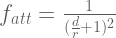
After looking at the results from a series of tests, it became apparent that the attenuation of a spherical light can be modeled as:

where:
d = distance between the light’s surface and the point being shaded
r = the light’s radius

Expanding this out, we get:

which is the original point light attenuation equation with the following attenuation factors:

Below are a couple of renders of four lights above a plane. The first is a ground-truth render of direct illumination calculated using Monte Carlo integration:

In this second render, direct illumination is calculated analytically using the attenuation factors derived from the light radius:

The only noticeable difference between the two is that in the second image, an area of the plane to the far left is slightly too bright due to a lack of a shadowing term.

Maybe this is old news to many people, but I was pretty happy to find out that an equation that had seemed fairly arbitrary to me for so many years actually had some physical motivation behind it. I don’t really understand why this relationship is never pointed out, not even in Foley and van Dam’s venerable tome*.

Unfortunately this attenuation model is still problematic for real-time rendering, since a light’s influence is essentially unbounded. We can, however, artificially enforce a finite influence by clipping all contributions that fall below a certain threshold. Given a spherical light of radius r and intensity Li, the illumination I at distance d is:

Assuming we want to ignore all illumination that falls below some cutoff threshold Ic, we can solve for d to find the maximum distance of the light’s influence:

Biasing the calculated illumination by -Ic and then scaling by 1/(1-Ic) ensures that illumination drops to zero at the furthest extent, and the maximum illumination is unchanged.

Here’s the result of applying these changes with a cutoff threshold of 0.001; in the second image, areas which receive no illumination are highlighted in red:

And here’s a cutoff threshold of 0.005; if you compare to the version with no cutoff, you’ll see that the illumination is now noticeably darker:

Just to round things off, here’s a GLSL snippet for calculating the approximate direct illumination from a spherical light source. Soft shadows are left as an exercise for the reader.

vec3 DirectIllumination(vec3 P, vec3 N, vec3 lightCentre, float lightRadius, vec3 lightColour, float cutoff)
{
    // calculate normalized light vector and distance to sphere light surface
    float r = lightRadius;
    vec3 L = lightCentre - P;
    float distance = length(L);
    float d = max(distance - r, 0);
    L /= distance;
    
    // calculate basic attenuation
    float denom = d/r + 1;
    float attenuation = 1 / (denom*denom);
    
    // scale and bias attenuation such that:
    //   attenuation == 0 at extent of max influence
    //   attenuation == 1 when d == 0
    attenuation = (attenuation - cutoff) / (1 - cutoff);
    attenuation = max(attenuation, 0);
    
    float dot = max(dot(L, N), 0);
    return lightColour * dot * attenuation;
}

* I always felt a little sorry for Feiner and Hughes.

Advertisement