Spherical harmonics, WTF?
April 14, 2011
I never really “got” spherical harmonics, there was something about them that just didn’t click for me. A little late to the party, I spent a few evenings recently reading over all the introductory papers I could find. Several times. This post is mostly just a brain dump, made in an effort to get everything straighted out in my head. I did stumble across a few curiosities though…
Real valued spherical harmonics can be defined as:

Where…

etc…


Assuming points on a unit sphere are defined in Cartesian coordinates as:


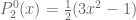
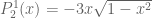
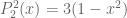
Then the first three bands of the SH basis are simply:


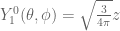
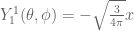
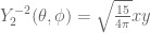
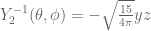
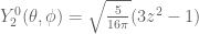
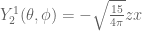
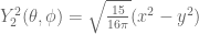
Note the change in sign of odd m harmonics, which is consistent with the above definitions of x, y, z and P. In many sources the basis function constants are all positive, which can be explained by assuming that they’re defined using the Condon-Shortley phase. That took me a while to figure out.
Projecting incident radiance L into the SH basis is done using the following integral:

This is actually a spectacularly bad approximation for low numbers of SH bands. For example, here’s Paul Debevec’s light probe of Grace cathedral:

And here’s that same probe’s projection into three SH bands (negative values have been clamped to zero):

Wow.
Fortunately, while spherical harmonics aren’t generally good at representing incident radiance, they totally kick arse at representing irradiance. (Very roughly speaking, incident radiance is the the amount of light falling on a surface from a particular direction, while irradiance is the total sum of light falling on a surface from all directions.)
In SH form the conversion from radiance L to irradiance E is marvelously simple:
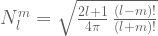
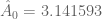
The definition of A isn’t exactly straight forward, but luckily smart people have already done the hard work for us:


The fact that terms after 2 fall off very quickly is what makes it possible to approximate irradiance fairly accurately with only three bands.
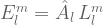
Given a set of spherical harmonic irradiance coefficients, the diffuse illumination for a particular direction is calculated by:

Condon-Shortley phase aside, something else that confused me were the results from An Efficient Representation for Irradiance Environment Maps. As far as I can tell, the gamma is not correct for some (possibly all) of the images in that paper, which made comparing results from my own code frustrating. The problems are compounded by the fact that the authors chose to apply some undefined tone mapping operator to some images, but not others.
Here’s the Grace cathedral probe again, this time with an exposure of -2.5 stops:

Below is the result I got from performing a diffuse convolution of the probe using Monte Carlo integration and 1024 samples per pixel (I was too impatient to wait for a brute force convolution to finish). The exposure is set to -2.5 stops. It’s very close to the result of applying a diffuse convolution in HDR Shop:

And here’s the result of projecting the light probe into three SH bands and converting from the coefficients from radiance to irradiance. Again, the exposure is -2.5 stops. It’s pretty close to the Monte Carlo result, which is reassuring:

Now, let’s compare these results to the those from the irradiance environment maps paper. First, their brute force diffuse convolution:

And now their SH approximation:

My guess is that they either applied a gamma curve of 2.2 for some reason, or didn’t correctly account for sRGB colour space when performing the HDR to LDR conversion. Or am I doing it wrong?
Here are the papers that I cribbed from:
Ramamoorthi & Hanrahan’s paper that introduced SH to the rendering community: An Efficient Representation for Irradiance Environment Maps
Their earlier paper actually contains a more rigorous treatment of spherical harmonics: On the relationship between radiance and irradiance: determining the illumination from images of a convex Lambertian object
Robin Green’s great introduction to the topic: Spherical Harmonic Lighting: The Gritty Details
And Volker Schönefeld wrote my favourite introduction, the way he describes SH in terms of separate functions of theta and phi made everything fall into place: Spherical Harmonics
